Bayesian Modeling Using WinBUGS: An introduction
by Ioannis Ntzoufras.


by Ioannis Ntzoufras.
News
- [1/2/2012] Erratum 3 was updated with more corrections.
- [1/2/2012] A problem with the data in Example 9.4 was corrected. Correct pages 319-321 were uploaded.
- [1/2/2012] A link to the review of Christian Robert was added.
- [1/2/2012] The expression for the variance of Zero inflated models was corrected. The correct code was uploaded. Special thanks to Gheorghe Doros for tracing this mistake]
- [13/7/2011] Some minor corrections were added in errata.
- [2/5/2011] A second edition will be out until 2013 including an introductory chapter for categorical data, a chapter for some more advanced models and reference to openbugs.
- [2/5/2011] Two minor corrections were added in errata.
- [17/9/2010] A correction for the code in page 328 was added.
- [6/7/2010] WORKSHOP ON BAYESIAN MODELLING USING WINBUGS
- [6/7/2010] Corrections I collected over the last 6 months were added in the Erratum of the 3rd edition.
- [26/2/2010] Some more corrections were found and send by readers and will be added soon.
- [25/2/2010] A 7 page review for my book in the Journal of Mathematical Psychology (see below for details).
- [11/2/2010] Honorable Mention (2nd Place) for the BOOK (Bayesian Modeling Using WinBUGS) in Subject of Mathematics in PROSE AWARDS for 2009; see for details here http://www.proseawards.com/current-winne
rs.html. Distinctions and Reviews
[07/11/2011] Review in Cristian Robert's blog.
[25/2/2010] A 7 page review for my book in the Journal of Mathematical Psychology:
Wetzels, R. & Wagenmakers, E.-J. (in press). Exemplary Introduction to Bayesian Statistical Inference. Book review of "Bayesian Modeling Using WinBUGS" (Wiley, 1st ed., 2009). Journal of Mathematical Psychology. available at http://www.ruudwetzels.com/articles/BMW_review.pdf .
[20/2/2010] Review from P. Turk in Pillows Blog.
[11/2/2010] Honorable Mention (2nd Place) for the BOOK (Bayesian Modeling Using WinBUGS) in Subject of Mathematics in PROSE AWARDS for 2009; see for details her http://www.proseawards.com/current-winne
rs.html. [1/10/2010] Two customer reviews in Amazon.com [5 stars]
[3/11/2010] One customer review in Amazon.co.uk.[3 stars]
Downloads
- Log of the web page.
- Errata [Updated 1/2/2012].
- Table of contents [pdf file].
- List of all examples and problems [pdf file].
- Index of all examples (by subject) [pdf or jpg file].
- Index of all examples (by dataset/problem) [pdf or jpg file].
- All files [zipped file; 5096 KB, updated 1/2/2012]
- All examples data [zipped Rdata or R source file - version 2.3.1 or higher].
- Brief guidance for selection of initial values [added 13/3/2009].
- Readers' questions [added 7/7/2009].
Related links
- The WinBUGS project.
- Postgraduate Course: Bayesian Statistics Using BUGS
- Tutorial: Introduction to MCMC and BUGS
- Other WinBUGS courses
Note
To download the (WinBUGS) odc files click the right mouse (on the appropriate link) button and then select "Save Target As..."Detailed list of examples
Chapter 1
1.1: Bayes theorem in case control studies [imaginary data]; see page 4.
1.2: Goals scored by the national football team of Greece in Euro 2004 (Poisson data); see page: 15.
Dataset: goals of the national Greek team in Euro 2004 (see book index).
Source: data are publicly available on the web
Download: Data [in text format] & R code (including data).
1.3: Estimating the prevalence of a disease (Bernoulli data). [imaginary data]; see page: 18.
Download: R code (including data).
1.4: Kobe Bryant's field goals in NBA (Binomial data); see page: 19.
Dataset: Kobe Bryant's field goals in NBA.
Source: Yahoo Sports.
Download: Data [in text format] [in R (dump) format] & R code [data are loaded from the corresponding R file].
1.5: Body temperature data (Normal data); see page: 21.
Dataset: Body temperature data (see book index).
Source: Shoemaker, A. L. (1996), What's normal? - temperature, gender, and heart rate, Journal of Statistics Education, 4 (2), available at http://www.amstat.org/publications/jse/v4n2/datasets.shoemaker.html.
Download:Data [in text format] [in R (dump) format]
R code
File 1: Low-information prior.
File 2: informative prior.
File 3: sensitivity analysis.
Chapter 2
2.1: A simple example: risk measures in medical research [imaginary data]; see page: 33.
Download: R code (including data).
2.2: Univariate example: Posterior distribution of the odds and log-odds in Binomial data; see page: 46.
Dataset: Kobe Bryant's field goals in NBA (see example 1.4).
Download: R code [for random walk and posterior analysis (including data)].
2.3: Univariate example: Posterior distribution of the odds and log-odds in Binomial data; see page 56.
Dataset: Senility symptoms data (or WAIS data).Source: Agresti, A. (1990), Categorical Data Analysis, Wiley-Interscience, New York.
Data are reproduced with the permission of John Wiley and Sons, Inc.
Download: Data [in text format] [in R (dump) format] & R code [collection of files including an mcmc.output file].
2.4: Body temperature dataset revisited: Analysis with non-conjugate prior; see page 72.
Dataset: Body temperature data (see example 1.5).Download: R code.
2.5: Slice sampler for binary logistic regression: senility symptoms data revisited; see page 77.
Dataset: Senility symptoms data (see example 2.3).
Source: Agresti, A. (1990), Categorical Data Analysis, Wiley-Interscience, New York.
Data are reproduced with the permission of John Wiley and Sons, Inc.
Download: R code
File 1: MCMC.
File 2: Diagnostic plots.
Chapter 3
Section 3.4.7: An example of a complete model specification in WinBUGS; see page 107.
Dataset: simulated normal data.
Download: WinBUGS code (including data); see Section 3.4.7, pages 107-108.
Chapter 4
Section 4.1: A complete example of running MCMC in WinBUGS for a simple model; see page 125.
Dataset: Kobe Bryant's field goals in NBA (see example 1.4).
Download: WinBUGS code (including data); see Section 4.1, pages 125-127.
Chapter 5
5.1: Soft drink delivery times data; see page 157.
Dataset: Soft drink delivery times data.Source: Montgomery, D. and Peck, E. (1992), Introduction to Regression Analysis, Wiley, New York.
Data are used and reproduced with permission of John Wiley and Sons, Inc.Model: Normal regression
Download:
Data [in text format]
WinBUGS code (including data)
File 1: regression model using independent normal prior distributions; see Section 5.2.4, Tables 5.2-5.3, pages 158-159.
File 2: regression model using Zellner's g-prior; see Section 5.3.4, Tables 5.5, page 165.
File 3: regression model expression with conjugate normal gamma prior; see Section 5.2.4, Tables 5.6, page 166.
5.2: Evaluation of candidate school tutors [imaginary data]; see page 171.
Model: One-way ANOVA.
Download: WinBUGS code (including data); see Section 5.4.4, Table 5.11, page 172.
5.3: Schizotypal personality data; see page 178.
Dataset: Schizotypal personality data.Source: the data were simulated from the group means of Iliopoulou, K. (2004), Schizotypy and Consumer Behavior (in Greek), Master's thesis, Department of Business Administration, University of the Aegean, Chios, Greece,
available at http://stat-athens.aueb.gr/~jbn/courses/diplomatikes/business/Iliopoulou(2004).pdf.
Model: Two-way ANOVA.Download: WinBUGS code (including data).
File 1: Two-way ANOVA model with no missing values (tabular data format and tabular model definition); see Section 5.4.5.5, Table 5.15, page 180.
File 2: Two-way ANOVA model with no missing values using (individual data with missing values); see Section 5.4.5.5, pages 182-184.
Chapter 6
6.1: A three-way ANOVA model for schizotypal personality data; see page 191.
Dataset: Schizotypal personality data; see example 5.3.
Source: Iliopoulou (2004); see example 5.3 for details.
Model: Three-way ANOVA.Download: WinBUGS code (including data).
File 1: Saturated three-way ANOVA with dummy variables; see Section 6.1, Table 6.2, page 193.
File 2: Saturated three-way ANOVA with dummy variables and likelihood specification using matrices and vectors; see Section 6.1, Tables 6.3, page 194.
File 3: Reduced three-way ANOVA with dummy variables and likelihood specification using matrices and vectors (without specific higher order interaction terms; see Section 6.1, Results of this model are presented in Table 6.5, pages 195-196.
6.2: Bioassay - Factor 8 blood clotting times example [imaginary data]; see page 204.
Model: ANCOVA.
Download: WinBUGS code (including data)
Model 1: Parallel lines model.
File 1: Simple ANCOVA model with parallel lines; see Section 6.3.1, Table 6.7, page 206].
File 2: As file 1 with log2-dose as explanatory; see Section 6.3.1, see for results in Tables 6.10, page 208-210.
File 3: As file 1 using dummies only for treatment; see Section 6.1.
File 4: As file 1 using design matrix and dummies; see Section 6.3.1, Table 6.8, page 207.
Model 2: Separate regression lines. This model was used to check the assumption of parallel lines in Model 1. It appears as (2 Non common slope) in Table 6.16, page 218.
File 5: Simple ANCOVA model with different intercepts and slopes; see Section 6.3.3, pages 1F7-218.
File 6: As file 5 with log2-dose as explanatory.
File 7: As file 5 with design matrix/dummies.
File 8: As file 7 with log2-dose as explanatory.
Model 3: Parallel lines model.
File 9: Simple ANCOVA model common intercept and different slopes; see Section 6.3.2, Table 6.12, page 214.
File 10: As file 9 with design matrix/dummies; see Section 6.3.2, Table 6.13, page 215.
Model 4: Non-common intercept model. This model was used to check the assumption of common intercept in Model 3. It appears as (4 Non common intercept) in Table 6.16, page 218.
File 11: ANCOVA model with non-common intercepts and different slopes; see Section 6.3.3, pages 217-218.
File 12: As file 11 with design matrix/dummies.
6.3: Oxygen uptake experiment; see page: 221.
Dataset: Oxygen uptake experiment data
Source: Weisberg, S. (2005), Applied Linear Regression, 3rd ed., Wiley-Interscience, New York, p.230-231.
Data are used and reproduced with permission of John Wiley and Sons, Inc.
Analysis: Stepwise variable selection using DIC in Regression. A number of p=5 models are fitted in parallel in each step in order to evaluate which variables must be included or excluded from the model using DIC.
Download: WinBUGS code (including data); see Section 6.4.3.1, pages 222-223. [Updated 21/7/2009]
Chapter 7
7.1: Aircraft damage example; see page: 245.
Dataset: Aircraft damage dataset
Source: Montgomery, D., Peck, E. and Vining, G. (2006), Introduction to Linear Regression Analysis, 4th ed., Wiley, Hoboken, NJ.
Data are used and reproduced with permission of John Wiley and Sons, Inc.
Model: Poisson Regression.
Download:
Data [in text format]
WinBUGS code (including data); see section 7.4.2, pages 245-249.
File 1: Poisson regression model and profiles.
File 2: Code for stepwise variable selection using DIC [Updated 21/7/2009].
7.2: Modeling the English Premiership football data; see page: 249.
Dataset: English Premiership data for the season 2006-2007
Source: http://soccernet-akamai.espn.go.com.
Model: Poisson log-linear.
Download:
Data [in R source format]
WinBUGS code (including data).
File 1: Poisson log-linear model for soccer data; see Section 7.4.3.2, page 250.
File 2: As in file 1 with prediction of two games; see Section 7.4.3.4, pages 251-253.
File 3: As in file 1 with regeneration of the full league; see Section 7.4.3.5, pages 253-255.
File 4: Negative binomial model [this is not included in the book - the theory and an example for the negative binomial model can be found in section 8.3.1, pages 283-286].
7.3: Analysis of senility symptoms data using WinBUGS; see page: 263.
Dataset: Senility symptoms data (see example 2.3).
Source: Agresti, A. (1990), Categorical Data Analysis, Wiley-Interscience, New York.
Data are reproduced with the permission of John Wiley and Sons, Inc.
Model: Binary response models (logit/probit/clog-log).
Download: WinBUGS code (including data) [Code for logit, probit and clog-log models]; see Section 7.5.2, pages 263-267.
Chapter 8
8.1: An inverse Gaussian simulated dataset; see page 278
Dataset: Simulated data.
Model: Inverse Gaussian model.
Download: WinBUGS code (including data) [Code for using zeros or ones trick]; see Section 8.1.2, pages 278-279, Table 8.2.
8.2: Soft drink delivery data (example 5.1 revisited); see page 281.
Dataset: Soft drink delivery times data; see example 5.1.
Source: Montgomery, D. and Peck, E. (1992), Introduction to Regression Analysis, Wiley, New York.
Data are used and reproduced with permission of John Wiley and Sons, Inc.Models: Models for positive continuous responses ( log-normal, gamma, exponential, chi square, inverse gamma and Weibull models)
Download: WinBUGS code (including data) [Code for normal, log-normal, gamma, exponential, chi square, inverse gamma and Weibull models]; see Section 8.2.3, pages 281-282.
8.3: 1990 USA general social survey - number of monthly sexual intercourses; see page 284
Dataset: 1990 USA general social survey data
Source: Agresti, A. (2002), Categorical Data Analysis, 2nd ed., Wiley-Interscience, Hoboken, NJ, p. 569–570.Data are used and reproduced with permission of JohnWiley and Sons, Inc.
Download:
Data [grouped, in txt format] [in R source format]
Model 1: Negative binomial model.
WinBUGS code (including data) [Code for (a) negative binomial - GLM formulation, (b) negative binomial - simpler representation, (c) Poisson log-linear model]; see Section 8.3.1, pages 284-286.
R code for (a) formatting data for WinBUGS and (b) calculation of DIC (see Table 8.5, page 286).
Model 2: Generalized Poisson model.
WinBUGS code (including data); see Section 8.3.2, pages 286-287.
File 1 - individual data.
File 2 - grouped data.
Model 3: Zero inflated models.
WinBUGS code (including data); see Section 8.3.3, pages 288-291.
File 1 - ZIP model. [Corrected 1/2/2012]
File 2 - ZINB model. [Corrected 1/2/2012]
File 3 - ZIGP model.[Corrected 1/2/2012]
[The variance expression was corrected in the above files on 1/2/2012; Thanks to Gheorghe Doros for tracing this mistake]
R code for DIC calculation (see Table 8.6, page 291 for results). [Updated 7/10/2009]
8.4: Bivariate simulated count data; see page 293.
Dataset: Bivariate Poisson simulated data.
Model: Bivariate Poisson model.
Download: WinBUGS code (including data); see Section 8.3.4, pages 291-293.
File 1- code using both zeros trick and Poisson.
File 2 - code using only zeros trick; code for the full and true model are available in both files.
8.5: Analysing the differences of bivariate count data; page 296.
Dataset: Bivariate Poisson simulated data of example 8.4.
Model: Poisson difference model (Skellam's distribution).
Download: WinBUGS code (including data) [code for the full and true model are available in both files]; see Section 8.3.5, pages 293-296.
Additional example 8.6: Agresti's (2000) Aligators data; see page 300.
Dataset: Alligators dataset.
Source: Agresti, A. (2002), Categorical Data Analysis, 2nd ed., Wiley-Interscience, Hoboken, NJ, p. 569–570.
Data are used and reproduced with permission of JohnWiley and Sons, Inc.
Models: Multinomial and Binomial Models.
Download: WinBUGS code (including data) [Code for (1) using dcat, (2) using multinomial, (3) using separate binomials, (4) using separate logistic regression models and (5) using two separate conditional logistic regression models.
Data [in text format]
Additional example 8.7: Agresti's (2000) political party data; see page 300. [ADDED 9/3/2009]
Dataset: Political party data.
Source: Agresti, A. (2002), Categorical Data Analysis, 2nd ed., Wiley-Interscience, Hoboken, NJ, p. 569–570.
Data are used and reproduced with permission of JohnWiley and Sons, Inc.
Models: Multinomial and Binomial Models.
Download: WinBUGS code (including data) [Code for (1) using multinomial, (2) using Poisson log-linear models.
Data [in text format]
Chapter 9
9.1: Repeated measurements of blood pressure [imaginary data]; see page 308.
Models: Simple hierarchical/random effects and fixed effects models.
Download: WinBUGS code (including data); see Section 9.2.1, pages 308-312.
File 1- simple hierarchical & corresponding multivariate model.
File 2 - constant model.
File 3 - hierarchical, constant and fixed effects models with missing values.
9.2: Random effects models for Kobe Bryant’s data; see page 313.
Dataset: Kobe Bryant's field goals in NBA (see example 1.4).
Models: Hierarchical/random effects, State space and fixed effects models.
Download: WinBUGS code (including data); see Section 9.2.2, pages 313-315.
File 1- simple hierarchical & fixed effects model.
File 2 - state space model.
9.3: Poisson mixture model for 1990 USA general social survey data; see page 315.
Dataset: 1990 USA general social survey data; see example 8.3.
Source: Agresti, A. (2002), Categorical Data Analysis, 2nd ed., Wiley-Interscience, Hoboken, NJ, p. 569–570.Data are used and reproduced with permission of JohnWiley and Sons, Inc.
Models: Poisson Mixture models (Poisson-gamma and Poisson-log-normal models).
Download: WinBUGS code (including data); see Section 9.2.3, pages 315-317.
File 1- Negative binomial model using Poisson-gamma representation.
File 2 - Poisson-log-normal model].
9.4: Meta-analysis example - analysis of odds ratios from various studies [imaginary data]; see page 319.
Models: Hierarchical model for meta-analysis.
Download: WinBUGS code (including data); see Section 9.2.4, pages 319-320. [CORRECTED CODE, 1/11/2009, Corrected Data 1/2/2012]
Corrected pages 319-321 of example 9.4 [ADDED 1/11/2009, Corrected 1/2/2012]
9.5: An AB/BA cross-over trial; see page 322.
Dataset: AB/BA cross-over trial data.
Source: Brown, H. and Prescott, R. (2006), Applied Mixed Models in Medicine, Statistics in Practice, 2nd ed., Wiley, Chichester, UK, p.275–279.
Data are used and reproduced with permission of JohnWiley and Sons, Inc.
Models/Analysis: Fixed and random effects models.
Download:
Data [in txt format]
WinBUGS code (including data); see Section 9.3.1, Table 9.8 and pages 321-325.
Model 1: Fixed effects and no baseline.
Model 2: Random effects and no baseline.
Model 3: Fixed effects with baseline measurement.
Model 4: Random effects with baseline measurement.
Model 5: Model 4 with carry-over effects.
Model 6: Random effects with baseline but no period effect.
Models 1-4 (with gamma indicators): Code for fitting models 1-4 by defining gamma binary indicators (normal model).
Log-normal models 1-4: Code for fitting models 1-4 by defining gamma binary indicators (log-normal model).
9.6: Treatment comparison in matched-pair clinical trials [imaginary data]; see page 327.
Models/Analysis: Conditional logistic regression using a simple random intercept model.
Download: WinBUGS code (including data); see Section 9.3.2.1, Table 9.12 and pages 326-329.
Model 1: Random intercept (individual effect) model.
Model 2: Constant model (same probability for all individuals).
Model 3: Constant probability for each each measurement.
9.7: Modeling correlation in schizotypal personality questionnaire binary responses; see page 329.
Dataset: Schizotypal personality data.
Source: Iliopoulou, K. (2004), Schizotypy and Consumer Behavior (in Greek), Master's thesis, Department of Business Administration, University of the Aegean, Chios, Greece, available at http://stat-athens.aueb.gr/~jbn/courses/diplomatikes/business/Iliopoulou(2004).pdf.
Models/Analysis: Logit GLMM for questionnaire data.
Download: WinBUGS code (including data); see Section 9.3.2.1, pages 329-332.
Model 1: Random intercept (individual effect) model; see Table 9.14, page 330.
Model 2: Constant model (same probability for all individuals).
9.8: Modeling water polo world cup 2000 data; see page 334.
Dataset: Water Polo world cup 2000 data.
Source: Data are publicly available at the web.
Models/Analysis: Poisson log-linear GLMM.
Download: WinBUGS code (including data); see Section 9.3.3, pages 333-337.
Model 1: Fixed effects model.
Model 2: Individual random effects (modeling overdispersion); see Table 9.18, page 335.
Model 3: Game random effects (modeling correlation).
Model 4: Phase and game random effects (modeling correlation, overdispersion and clustering)
Model 5: Individual, phase and game random effects (modeling correlation, overdispersion and clustering).
Chapter 10
10.0: Estimating missing observations; see page 345.
Dataset: Schizotypal personality data; see example 5.3.
Source: the data were simulated from the group means of Iliopoulou, K. (2004), Schizotypy and Consumer Behavior (in Greek), Master's thesis, Department of Business Administration, University of the Aegean, Chios, Greece,available at http://stat-athens.aueb.gr/~jbn/courses/diplomatikes/business/Iliopoulou(2004).pdf.
Model: Two-way ANOVA (with missing values).Download: WinBUGS code (including data)
File 0 - normal model on the logarithms of Y with transformed data [does not work unless full data are used]. [UPDATED 2/6/2009]
File 1 - normal model on the logarithms of Y [data must be loaded in log-scale]. [ADDED 2/6/2009]
File 2 - using log-normal model on Y.
10.1: Outstanding car insurance claim amounts; see page 347
Dataset: Insurance claim amount data
Source: Ntzoufras, I. and Dellaportas, P. (2002), Bayesian modelling of outstanding liabilities incorporating claim count uncertainty (with discussion), North American Actuarial Journal 6, 113–128.
Copyright 2002 by the Society of Actuaries, Schaumburg, Illinois. Reproduced and reprinted with permission.Also available in Ntzoufras, I. (1999), Aspects of Bayesian Model and Variable Selection Using MCMC, PhD thesis, Department of Statistics, Athens University of Economics and Business, Athens, Greece, available at http://stat-athens.aueb.gr/~jbn/publications.htm.
Model: Two-way log-normal ANOVA model (with missing values).
Download: WinBUGS code (including data); see Section 10.2.2, Table 10.6, page 351.
10.2: The distribution of Manchester United’s goals in home games for season
2006-7; see page 354.
Dataset: Manchester United's goals.Source: Data are publicly available at the web.
Model/Analysis: Predictive measures for a simple Poisson model (predictive frequencies, posterior predictive ordinates (PPOs), conditional predictive ordinates (CPOs) & posterior p-values).
Download: WinBUGS code (including data)
File 1 - calculation of predictive frequencies (see page 355 for code, 356 for results)
File 2 - calculation of PPO (see page 360 for code, 360-361 for results); calculation of posterior p-value for overdispersion (see page 366 for code and results); posterior p-values based on χ2 (see pages 368-371 for code and results); conditional predictive ordinates (CPO) (see page 376 for code and results).
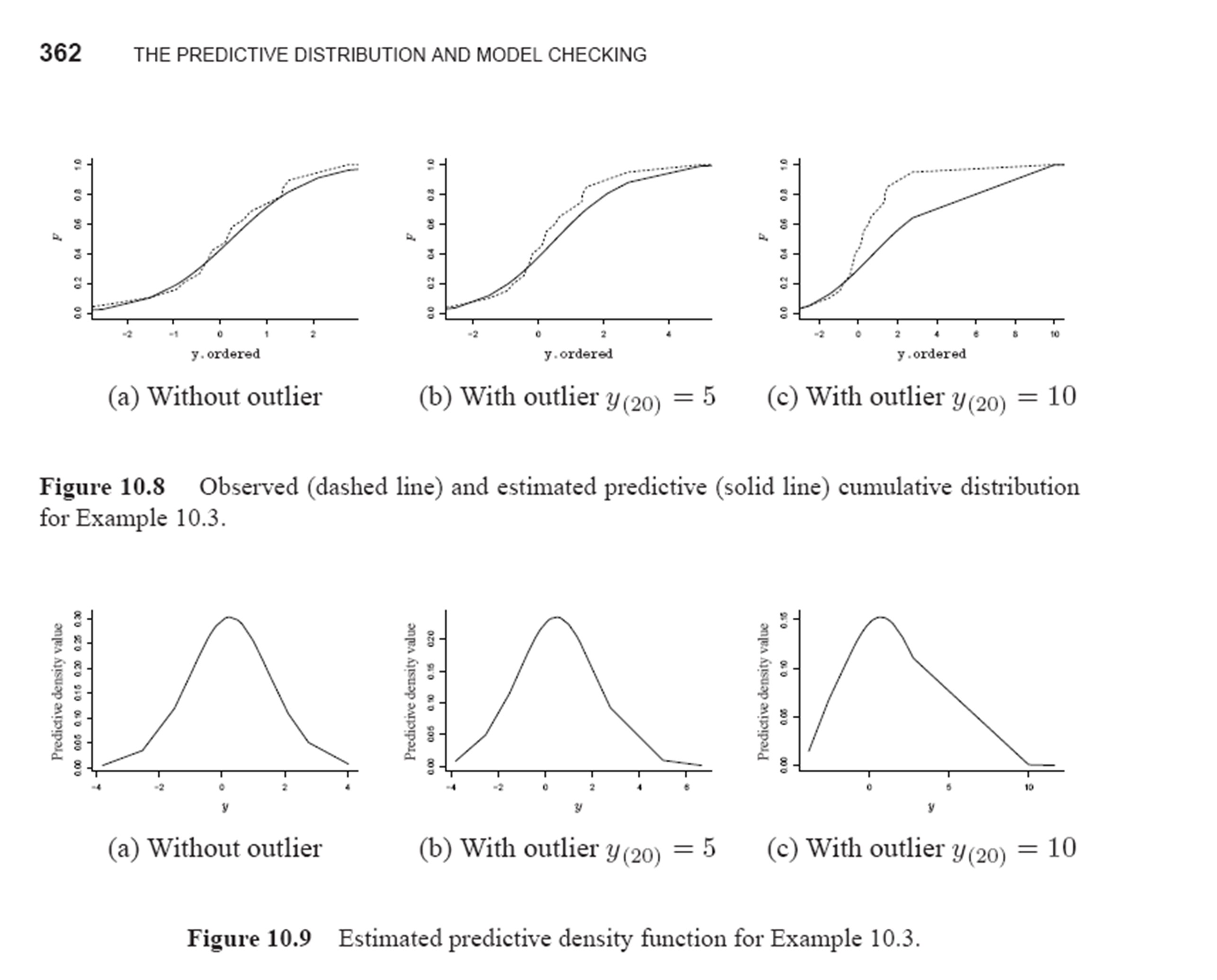
10.3: Simulated normal data; see page 357.
Dataset: Simulated normal data.Model/Analysis: Predictive measures for a simple normal model (predictive cumulative frequencies, ordered predictive data, posterior predictive ordinates (PPOs), conditional predictive ordinates (CPOs) & posterior p-values).
Download: WinBUGS code (including data)
File 1 - calculation of predictive cumulative frequencies (see page 357 for code, 357-358 for results) ordered predictive data (see page 358-359 for results); PPOs (see page 361-362 for code and results); posterior p-values for kurtosis and symmetry (see pages 366-368 for code and results); CPOs and PPOs (see page 377 for results). [CORRECTED AND UPDATED 8/6/2009]
File 2 - residuals.
File 3 - posterior p-values based on χ2 measures (see pages 371-374 for code and results).
10.4 : Model checking for the soft drink delivery times data (Example 5.1 continued); see page 383.
Dataset: Soft drink delivery times data; see example 5.1.Source: Montgomery, D. and Peck, E. (1992), Introduction to Regression Analysis, Wiley, New York.
Data are used and reproduced with permission of John Wiley and Sons, Inc.Model/Analysis: Predictive checks for a normal regression model.
Download: WinBUGS code (including data); see Section 10.5.5; pages 383-386.
Chapter 11
11.1: Calculation of the marginal likelihood in a beta binomial model - Kobe Bryant’s field goals in NBA (revisited); page 399.
Dataset: Kobe Bryant's field goals in NBA (see example 1.4).Model/Analysis: Calculation of the marginal likelihood for a simple beta-binomial model.
Download: WinBUGS code (including data); see Section 11.4.1; pages 399-402.
Model 1 - different success probabilities for each season.
Model 0 - common success probability for all seasons.
11.2: Calculation of the marginal likelihood in a normal conjugate model - Soft Drink Delivery Times (revisited); see page 403.
Dataset: Soft drink delivery times data; see example 5.1.
Source: Montgomery, D. and Peck, E. (1992), Introduction to Regression Analysis, Wiley, New York.
Data are used and reproduced with permission of John Wiley and Sons, Inc.Model/Analysis: Calculation of the marginal likelihood for a simple beta-binomial model.
Download:
WinBUGS code (including data); see Section 11.4.2, pages 403-405.
Model 1 - constant model.
Model 2 - cases as covariate.
Model 3 - distance as covariate.
Model 4 - cases & distance as covariates.
Model 4 - multivariate importance density for the generalized harmonic mean estimator
R code
File 1 - exact calculation of the marginal likelihood.
File 2 - calculation of marginal likelihood using the Laplace-Metropolis approach.
11.3: Bayesian Variable Selection in Dellaportas et al. (2002) simulated data; see page 414.
Dataset: Dellaportas et al. simulated data.
Source: Dellaportas, P., Forster, J. and Ntzoufras, I. (2002), On Bayesian model and variable selection using MCMC, Statistics and Computing 12, 27–36; with kind permission of Springer Science and Business Media.
Data are also available in Ntzoufras, I. (1999), Aspects of Bayesian Model and Variable Selection Using MCMC, PhD thesis, Department of Statistics, Athens University of Economics and Business, Athens, Greece, available at http://stat-athens.aueb.gr/~jbn/publications.htm.Model/Analysis: Variable selection methods for normal regression models.
Download:
Data [in txt format]
WinBUGS code (including data); see Section 11.7, pages 414-419.
Pilot run of the full model - used for the specification of the proposal parameters.
Prior 1 [full and reduced model space] - Independent normal priors (used in Dellaportas et al. 2002).
Prior 2 [full and reduced model space] - Zellner's g-prior.
Prior 3 [full and reduced model space] - Empirical based prior.
11.4: Posterior predictive densities for soft drink delivery times data; see page 424.
Dataset: Soft drink delivery times data; see example 5.1.
Source: Montgomery, D. and Peck, E. (1992), Introduction to Regression Analysis, Wiley, New York.
Data are used and reproduced with permission of John Wiley and Sons, Inc.Model/Analysis: Model evaluation using posterior predictive densities (normal regression models) - Posterior and pseudo-Bayes factors, leave-one-out cross-validation likelihood (cross-validatory predictive log-score), logarithmic score.
Download:
WinBUGS code (including data); see Section 11.10.2, page 424.
R code (for the computation of predictive measures from the MCMC output of WinBUGS model code); see Table 11.11, page 424 for results.
11.5: Calculation of AIC and BIC for soft drink delivery times data; see page 429.
Dataset: Soft drink delivery times data; see example 5.1.
Source: Montgomery, D. and Peck, E. (1992), Introduction to Regression Analysis, Wiley, New York.
Data are used and reproduced with permission of John Wiley and Sons, Inc.Download:
WinBUGS code (including data); see Section 11.11.6 pages 429-431.
R code (for the computation of the AIC and BIC from the MCMC output of WinBUGS model code); see Table 11.14, Figures 11.2 and 11.3, pages 430-431 for results.
Appendix A
Section A.5: A simple example of Doodle; see page 439.
Download: WinBUGS script code.
Appendix B
Section B.2: A simple script; see page 444.
Download: Script code and related files [in zip format]; unzip in C:\ otherwise change accordingly the directories in the script.odc file.
Appendix C
Section C.5.1: A simple example in CODA; see page 453.
Section C.5.2: A simple example in BOA; see page 457.
Download: .Rdata file and MCMC output files [in zip format].
PROBLEMS
Chapter 5
Problem 5.1: link to the Hubble's data story in DASL (Data and Story Library)
Problem 5.3: Dellaportas et al. (2002) data (see example 11.3 for details).
Download Data [in txt format]
Problem 5.7: link to the paper of Kahn (2005) and the associated dataset and description.
Problem 5.8: link to the Albuquerque home prices data story in DASL.
Chapter 6
Problem 6.9: MShop1 dataset.
Download Data [in txt format or in SPSS format]. Description of the variables is available here [or in txt format here]
Chapter 7
Problem 7.1: Simulated data. Download Data [in txt format].
Problem 7.2: MShop1 dataset; see Problem 6.9.
Problem 7.3: Water Polo data. Download Data [in S format].
Problem 7.4: Italian soccer/football championship data for season 2000-2001.
Download Data [in txt format or SPSS format].
Problem 7.7 Simulated data. Download Data [in txt format].
Figures
The following figures can be downloaded and printed in full color for higher clarity.
Figure 5.4.b Interaction plot based on posterior means of expected SPQ score in Example 5.3. [Download ps or pdf]
Figure 6.3 Graphical representation of parallel lines model using corner constrained parameters. [Download ps or pdf]
Figure 6.4 Graphical representation of separate regression lines model using corner constrained parameters. [Download ps or pdf]
Figures 10.8 & 10.9 Corrected Figures 10.8-10.9. [Download in jpg] [CORRECTED AND UPLOADED 8/6/2009]
All Contents Copyright.
Last revised: 16-05-2018